Sparse Matrix in Data Structures: Overview, Types & Examples

Table Of Content
- What is a Sparse Matrix in Data Structure?
- Why Do We Need Sparse Matrices?
- Types of Sparse Matrix
- Common Methods for Representing Sparse Matrices
India is experiencing a vibrant digital landscape, with over 900 million internet users, making it the second largest in the world. This tremendous growth in the digital world has also led to trillions of data generation, which further demands effective data management techniques. And this is where a Sparse matrix comes in. It is one of the most important techniques to optimise storage by mainly focusing on the nonzero elements rather than storing every element. Such matrices are used in multiple real-world applications, such as data science, machine learning, and graph theory, where data contains many zero values.
In this blog, we will delve deeper into what a sparse matrix is, its types, and examples. Stay tuned till the end of the blog to get only relevant information.
What is a Sparse Matrix in Data Structure?
 *engati.ai
 A sparse matrix is defined as a matrix where the number of zero elements is significantly larger than the number of non-zero elements. In layman’s terms, it has “more space than filled space.”
For example:
Matrix A =
[ 5 0 0 0 ]
[ 0 8 0 0 ]
[ 0 0 0 0 ]
[ 0 0 3 0 ]
Here, in the above 4*4 matrices, there are 16 total elements, 3 of the elements are non-zero, and the remaining 13 elements are zeros. Therefore, it is a sparse matrix.
Condition to Check Sparsity
A matrix is said to be sparse if:
Number of zero elements > Number of non-zero elements
Thus, if the matrix element contains mostly zeros, we use sparse matrix representation techniques to save memory.
Why Do We Need Sparse Matrices?
1. Memory Efficiency
- When a large matrix is regularly stored, it wastes memory by storing a lot of zero space.
- Sparse matrices only store the non-zero elements and the positions, which helps in terms of memory.
2. Computation Speed
When computing, such as addition, multiplication, and transposition, it is faster since you are only computing the non-zero portions.
3. Handling Large Data
- In certain fields, such as machine learning, computer animation, and specifically scientific simulators, their data is stored in large sparse matrices.
- Having an efficient means of storage can help manage some very large datasets that otherwise would not be useful to process.
Types of Sparse Matrix
1. Lower Triangular Sparse Matrix
A lower triangular sparse matrix is a special kind of square matrix in which all the elements above the main diagonal are zero, and the elements on or below the main diagonal can have non-zero values.
A lower triangular sparse matrix is a special kind of square matrix in which all the elements above the main diagonal are zero, and the elements on or below the main diagonal can have non-zero values.
Mathematically:
For a matrix Arr[i][j],
Arr[i][j] = 0 when i < j
In other words, all elements above the diagonal (upper-right part of the matrix) are zero.
Example:
Let’s take a 4×4 matrix:
Arr=
[ 3 0 0 0 ]
[ 4 2 0 0 ]
[ 1 7 5 0 ]
[ 6 8 9 4 ]
Here, every element above the main diagonal is 0, which makes it a lower triangular sparse matrix.
Number of Non-Zero Elements:
- 1 in the 1st row
- 2 in the 2nd row
- 3 in the 3rd row
- and so on…
So, for an n × n lower triangular matrix, the total non-zero elements = n(n + 1)/2.
Efficient Storage (One-Dimensional Mapping):
Instead of storing all the zero elements, we can map only the non-zero elements into a one-dimensional array. This saves memory.
There are two ways to store these elements:
- Row-wise mapping: Store row by row.
Example: {3, 4, 2, 1, 7, 5, 6, 8, 9, 4} - Column-wise mapping: Store column by column.
Example: {3, 4, 1, 6, 2, 7, 8, 5, 9, 4}
2. Upper Triangular Sparse Matrix
An upper triangular sparse matrix is the reverse of a lower triangular matrix. Here, all the elements below the main diagonal are zero, while the elements on or above the main diagonal may contain non-zero values.
Mathematically:
For a matrix Arr[i][j],
Arr[i][j] = 0 when i > j
Example:
Consider this 4×4 matrix:
[2 4 5 9]
[0 6 3 1]
[0 0 8 7]
[0 0 0 4]
All elements below the main diagonal are 0, making it an upper triangular sparse matrix.
Number of Non-Zero Elements:
- 4 in the 1st row
- 3 in the 2nd row
- 2 in the 3rd row
- 1 in the 4th row
So, total non-zero elements = n(n + 1)/2 (same as lower triangular).
Efficient Storage (One-Dimensional Mapping):
To optimise memory, only the upper triangular part is stored.
- Row-wise mapping: {2, 4, 5, 9, 6, 3, 1, 8, 7, 4}
- Column-wise mapping: {2, 6, 8, 4, 4, 3, 7, 5, 1, 9}
3. Tri-Diagonal Sparse Matrix
A tridiagonal sparse matrix is one in which the non-zero elements appear only on the main diagonal, the diagonal just above it, and the diagonal just below it. All other elements are zero.
Mathematically:
For a matrix Arr[i][j],
Arr[i][j] = 0 when |i – j| > 1
This means that elements are non-zero only when the column index and row index differ by at most 1.
Example:
Let’s consider a 5×5 matrix:
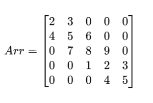
Here:
- The main diagonal: {2, 5, 8, 2, 5}
- The upper diagonal: {3, 6, 9, 3}
- The lower diagonal: {4, 7, 1, 4}
All other elements are 0.
Number of Non-Zero Elements:
- n elements on the main diagonal
- (n – 1) elements on the upper diagonal
- (n – 1) elements on the lower diagonal
So, total non-zero elements = 3n – 2.
Efficient Storage (Mapping Techniques):
Since only three diagonals have non-zero values, we can represent them compactly using a one-dimensional array in different ways:
- Row-wise mapping: {2, 3, 4, 5, 6, 7, 8, 9, 1, 2, 3, 4, 5}
- Column-wise mapping: {2, 4, 3, 5, 7, 6, 8, 1, 9, 2, 4, 3, 5}
- Diagonal-wise mapping: {4, 2, 7, 5, 8, 3, 9, 2, 1, 3, 4, 5}
Each of these mappings focuses only on the non-zero parts of the matrix, which makes it efficient for computation and storage.
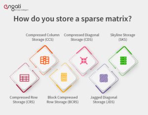
Common Methods for Representing Sparse Matrices
 *engati.ai
When working with sparse matrices, storing every zero element wastes a significant amount of memory. Instead, we only store the non-zero elements along with their positions in efficient data structures.
There are three widely used methods for sparse matrix representation:
1. Coordinate List (COO) Format
The Coordinate List (COO) format is one of the simplest and most intuitive ways to represent a sparse matrix. In this approach, we store each non-zero element along with its corresponding row index and column index.
Structure:
Each non-zero element is represented as a tuple:
(Row Index, Column Index, Value)
This format is particularly useful when:
- The sparse matrix is being constructed dynamically (e.g., during data input).
- The order of elements is not important.
- You need easy readability and debugging.
Example:
Consider the following 5×5 matrix:
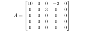
Here, only three elements are non-zero: 10, -2, and 3.
So, the COO representation is:
| Row | Column | Value |
| 0 | 0 | 10 |
| 0 | 3 | -2 |
| 1 | 2 | 3 |
Hence, the COO list becomes:
COO = [(0, 0, 10), (0, 3, -2), (1, 2, 3)]
Advantages:
- Easy to construct and modify.
- Ideal for building matrices incrementally.
2. Compressed Sparse Row (CSR) Format
The Compressed Sparse Row (CSR) format provides a more efficient and compact way to represent sparse matrices. It is especially suitable for operations that involve accessing rows, such as matrix-vector multiplication.
CSR uses three one-dimensional arrays to store information:
- Values[] – All non-zero elements in row-major order.
- ColumnIndex[] – The column index of each corresponding non-zero element.
- RowPointer[] – Index positions in the Values[] array where each new row starts.
Example:
Let’s use the same 5×5 matrix:
Step 1: Identify non-zero values
Values = [10, -2, 3]
Step 2: Record column indices
ColumnIndex = [0, 3, 2]
Step 3: Define row pointers
Each entry in RowPointer marks where a new row begins in the Values[] array.
RowPointer = [0, 2, 3, 3, 3, 3]
Here:
- Row 0 starts at index 0 and ends before index 2
- Row 1 starts at index 2 and ends before index 3
- Rows 2–4 have no non-zero values, so the pointer remains the same
CSR Representation:
Values = [10, -2, 3]
ColumnIndex = [0, 3, 2]
RowPointer = [0, 2, 3, 3, 3, 3]
Advantages:
- Very efficient for row slicing and matrix-vector multiplication.
- Saves substantial memory compared to COO.
3. Compressed Sparse Column (CSC) Format
The Compressed Sparse Column (CSC) format is similar to CSR but optimised for column-based operations.
It also uses three arrays, but the focus shifts from rows to columns:
- Values[] – All non-zero elements stored column-wise.
- RowIndex[] – The row index of each corresponding non-zero element.
- ColPointer[] – Index positions in Values[] where each new column starts.
Example:
Using the same matrix as above:
Step 1: Non-zero values (column-wise):
Values = [10, 3, -2]
Step 2: Record row indices:
RowIndex = [0, 1, 0]
Step 3: Define column pointers:
ColPointer = [0, 1, 1, 2, 3, 3]
CSC Representation:
Values = [10, 3, -2]
RowIndex = [0, 1, 0]
ColPointer = [0, 1, 1, 2, 3, 3]
Advantages:
- Ideal for column slicing or operations involving column-oriented algorithms.
- Memory-efficient and fast for certain mathematical operations (like solving linear systems).
Real-World Applications of Sparse Matrices
- Search Engines: Caches information on web pages and search terms in an efficient manner.
- Social Networks: Represent a user’s connections (friendships, followers) through the set of graph attributes, G=v,e.
- Machine Learning: Specific to recommendation engines (Netflix, Amazon, Spotify).
- Image Compression: Sparse matrices enable the seamless compression of images that contain large-scale blank areas.
- Scientific Computing: Widely used for the long and arduous process of solving linear equations and simulations.
Conclusion
In data structures, a Sparse Matrix is a very valuable idea that saves memory and computation time because it only looks at the non-zero values. Sparse Matrices are increasingly important in new applications such as search engines, recommendation engines, scientific computing, and big data analytics. Once we comprehend the alternatives available and understand the representations – triplet, CSR, CSC, and DOK – we can select the best representation for the problem at hand.
Also, if you want to get a foundational concept in AI, Mathematics, and Machine Learning, register for the Advanced Certificate Programme in ML, Gen AI & LLMs for Business Applications. The programme is designed to equip participants with the skills and knowledge required to harness the potential of Generative AI and Machine Learning.
Frequently Asked Questions
We represent sparse matrices in several different ways:
- Triplet form (row, column, value)
- Compressed Sparse Row (CSR)
- Compressed Sparse Column (CSC)
- Dictionary of Keys (DOK)
- Linked list representation

Find a Program made just for YOU
We'll help you find the right fit for your solution. Let's get you connected with the perfect solution.

Is Your Upskilling Effort worth it?

Are Your Skills Meeting Job Demands?

Experience Lifelong Learning and Connect with Like-minded Professionals

