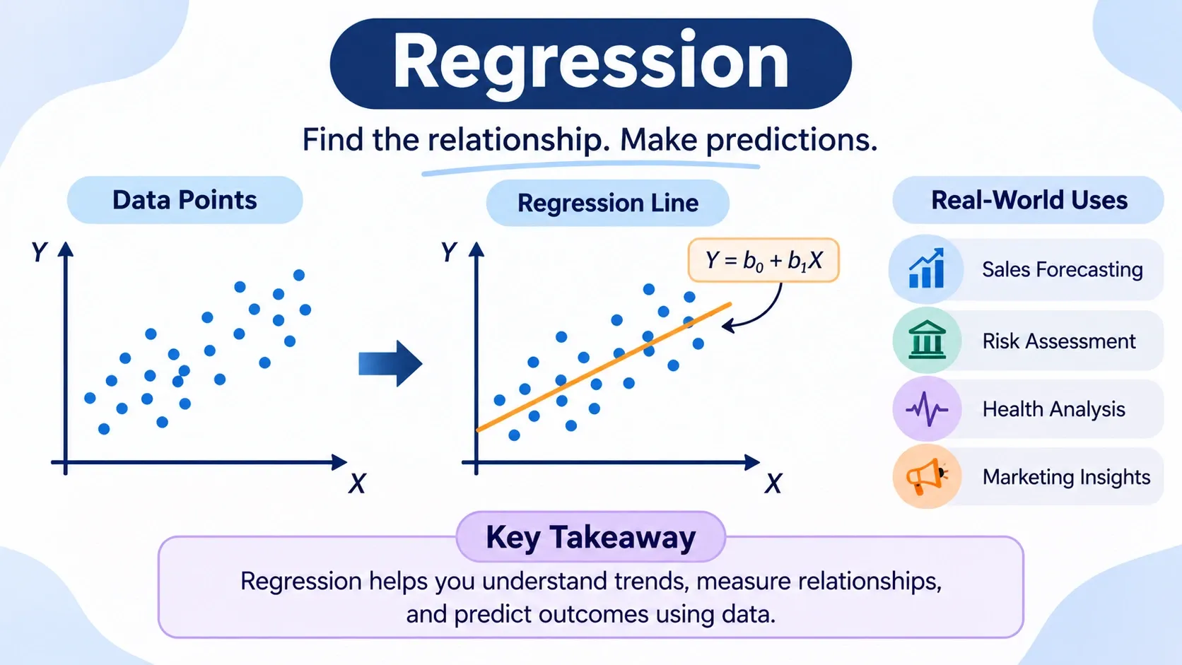
Regression is a statistical method used to understand relationships between dependent and independent variables, explain patterns, and predict future or unknown values.
Common types of regression include simple linear, multiple linear, polynomial, logistic, Ridge, and Lasso regression, each suited to different data and prediction needs.
Regression analysis involves defining the research question, collecting and cleaning data, fitting a model using the least squares method, checking R-squared and residuals, and testing assumptions.
Regression calculations use slope, intercept, and R-squared to measure relationships and evaluate how well a model explains variations in the outcome. Tools such as Excel, Google Sheets, Python, R, SPSS, and Stata can simplify these calculations.
In this blog, you'll learn the definition of regression, its types, key equations, calculation methods, a step-by-step example using study hours and exam scores, practical applications, and how to interpret regression results.
Have you ever wondered how a company predicts next quarter's sales, how a bank estimates the risk of a loan, or how a doctor judges the effect of a drug dose on blood pressure? Behind many of these predictions sits one of the most useful tools in statistics: regression. It turns scattered numbers into a clear relationship you can measure, test, and use.
If this subject interests you, it is also a strong foundation for a career in data. Many learners build these skills through structured study, such as anonline M.Sc. in Statistics from Dr. M.G.R. University, where applied regression analysis is part of the third-semester syllabus. Whether you are a student, an analyst, or just curious, this blog explains regression in plain language, shows how the math works, and walks through a complete example you can follow with a pencil and paper
Regression is a statistical method used to study the relationship between one outcome and one or more factors that may influence it. The outcome is called the dependent variable (or response). The factors are called independent variables (or predictors).
For example, a student’s exam score depends partly on the hours spent studying. Here, the exam score is the dependent variable and study hours is the independent variable. Regression helps you answer questions like:
Is there a relationship between the two?
How strong is it?
If study hours go up by one, how much does the score change on average?
Can we predict a score for a given number of study hours?
The word “regression” comes from the 1800s, when Sir Francis Galton noticed that children of very tall parents tended to be closer to average height than their parents. He called this “regression toward the mean.” The name stuck, even though modernregressioncovers much more than that original idea.
Regression is popular because it does three jobs at once.
Description: It summarizes how variables are connected.
Prediction: It estimates future or unknown values.
Explanation: It shows which factors matter most and by how much.
Businesses use it to forecast demand and set prices. Economists use it to study how interest rates affect spending. Healthcare researchers use it to link lifestyle habits with health outcomes. Marketers use it to measure the effect of advertising on sales. In machine learning, regression models are often the first approach people try because they are simple, fast, and easy to explain.
Types of Regression
Not every problem fits a straight line, so there are several kinds of regression. Here are the most common ones.
Simple linear regression. One predictor and one outcome, connected by a straight line. This is the starting point for most learners.
Multiple linear regression. Two or more predictors. For example, a house price may depend on area, number of bedrooms, and location.
Polynomial regression. Used when the relationship curves rather than following a straight line.
Logistic regression. Used when the outcome is a category, such as yes or no, pass or fail, buy or not buy. It predicts the probability of an event.
Ridge and Lasso regression. Variations that add a penalty to keep the model from becoming too complicated, which helps when there are many predictors.
The Regression Equation Explained
The simple linear regression equation looks like this:
Y = b0 + b1X
Y is the predicted value of the dependent variable.
X is the independent variable.
b0 is the intercept. It is the predicted value of Y when X is zero.
b1 is the slope. It tells you how much Y changes, on average, when X increases by one unit.
In practice, real data never falls perfectly on a line, so the full model includes an error term. That error represents everything the model does not capture, such as random variation or factors we did not measure.
The line is chosen using the least squares method. This method finds the line that makes the total of the squared gaps between actual values and predicted values as small as possible. Those gaps are called residuals.
Regression Analysis: Step-by-Step Process
Regression analysis is more than plugging numbers into a formula. A careful analyst follows a sequence of steps.
Define the question. Decide what you want to predict and which factors might affect it.
Collect and clean the data. Check for missing values, typing errors, and unusual entries.
Plot the data. A scatter plot quickly shows whether a straight-line relationship is reasonable.
Fit the model. Calculate the slope and intercept using the least squares method.
Check the fit. Look at R-squared and the residuals to see how well the model explains the data.
Test the assumptions. Make sure the model’s basic conditions are reasonable.
Interpret and use the results. Explain what the numbers mean in everyday language and make predictions carefully.
Free Courses
Free FinTech Course – FinTech 101: Digital Banking & Payments
Linear regression works best when certain conditions are roughly true. Checking them helps you avoid misleading results.
Linearity: The relationship between X and Y is approximately a straight line.
Independence: Each observation is independent of the others. One data point should not influence another.
Constant variance: The spread of residuals stays about the same across all values of X. Statisticians call this homoscedasticity.
Normal residuals: The residuals are roughly bell-shaped, which matters mostly for hypothesis tests and confidence intervals.
No severe multicollinearity: In multiple regression, predictors should not be too strongly correlated with each other.
You do not need perfection. Small departures are common, but large ones signal that the model needs a rethink.
Regression Calculation: The Formulas
The regression calculation for a simple linear model uses two formulas.
Slope: b1 = Σ(X − X̄)(Y − Ȳ) ÷ Σ(X − X̄)²
Intercept: b0 = Ȳ − b1 × X̄
Here, X̄ and Ȳ are the averages of X and Y. The top part of the slope formula measures how X and Y move together. The bottom part measures how spread out X is on its own.
To judge the quality of the fit, we also use R-squared (R²):
R² = 1 − (SSE ÷ SST)
SSE is the sum of squared residuals, which is the unexplained variation.
SST is the total variation in Y around its average.
R² ranges from 0 to 1. A value of 0.80 means the model explains about 80% of the variation in the outcome.
Regression Example: Study Hours and Exam Scores
Let us work through a complete regression example with real numbers. Suppose five students report their study hours and then receive their exam scores.
Student
Study Hours (X)
Exam Score (Y)
1
1
50
2
2
55
3
3
65
4
4
70
5
5
80
Step 1: Find the averages
X̄ = (1 + 2 + 3 + 4 + 5) ÷ 5 = 3
Ȳ = (50 + 55 + 65 + 70 + 80) ÷ 5 = 64
Step 2: Calculate the deviations
X
Y
X − X̄
Y − Ȳ
(X − X̄)(Y − Ȳ)
(X − X̄)²
1
50
−2
−14
28
4
2
55
−1
−9
9
1
3
65
0
1
0
0
4
70
1
6
6
1
5
80
2
16
32
4
Total
75
10
Step 3: Calculate the slope and intercept
b1 = 75 ÷ 10 = 7.5
b0 = 64 − (7.5 × 3) = 64 − 22.5 = 41.5
Step 4: Write the regression equation
Predicted Score = 41.5 + 7.5 × (Study Hours)
Step 5: Interpret the result
The slope of 7.5 means that, on average, each extra hour of study is linked to a 7.5-point increase in the exam score. The intercept of 41.5 is the predicted score for a student who studies zero hours. It is a useful anchor for the line, but be careful about reading too much into it when zero hours is outside the range of your data.
Step 6: Make a prediction
What score might we expect from a student who studies 3.5 hours?
Next, SST is the sum of squared differences between each Y and the average of 64: (−14)² + (−9)² + 1² + 6² + 16² = 196 + 81 + 1 + 36 + 256 = 570.
R² = 1 − (7.5 ÷ 570) = 1 − 0.0132 = 0.987
This means about 98.7% of the variation in exam scores is explained by study hours in this small sample. The correlation coefficient (r) is the square root of R², which is about 0.993, showing a very strong positive relationship.
A word of caution: this is a tiny, neat dataset built for teaching. Real data is messier, and an R² this high is rare outside textbooks.
How to Run Regression Using Common Tools
You rarely have to do the arithmetic by hand once you understand it. Here are a few easy ways to run a regression calculation.
Microsoft Excel or Google Sheets. Use =SLOPE(Y range, X range) for the slope, =INTERCEPT(Y range, X range) for the intercept, and =RSQ(Y range, X range) for R-squared. The LINEST function gives more detailed output.
Python. A short script with the scikit-learn library can fit the model:
from sklearn.linear_model import LinearRegression import numpy as np
X = np.array([[1], [2], [3], [4], [5]]) y = np.array([50, 55, 65, 70, 80])
model = LinearRegression().fit(X, y) print(model.intercept_, model.coef_[0]) # 41.5, 7.5
**R, SPSS, and Stata.** These are widely used in research and academic work, and they provide full statistical reports with a few commands.
Real-World Uses of Regression
Regression shows up in almost every field:
Finance: Estimating stock risk and forecasting returns.
Retail: Predicting sales based on price, season, and promotions.
Healthcare: Studying how age, weight, and habits relate to disease risk.
Real estate: Valuing homes using size, location, and amenities.
Education: Understanding how attendance and study habits affect results.
Marketing: Measuring how ad spend influences customer purchases.
Because it is simple to explain, regression is often the first model that analysts build before trying anything more complex.
Regression takes the question “how are these things connected?” and answers it with numbers you can test and use. You start with a scatter of data, fit a line using least squares, read the slope and intercept, and check how well the model explains the outcome. As the study hours example shows, the calculation itself is quite manageable once you break it into small steps.
The real skill lies in using it wisely: checking assumptions, avoiding the correlation versus causation trap, and keeping predictions within a sensible range. Start with simple linear regression, practice on small datasets, and then move on to multiple and logistic regression as your confidence grows.
Frequently Asked Questions
Correlation measures how strongly two variables move together and gives a single number between −1 and 1. Regression goes further by building an equation that predicts one variable from another. Correlation tells you the strength of a relationship, while regression tells you its form and lets you make predictions.
It depends on the field. In controlled physical sciences, an R² above 0.90 may be expected. In social sciences or human behavior studies, values of 0.30 to 0.60 can still be useful because people are harder to predict. A high R² alone does not prove a model is good, so always check residuals and think about the context.
Linear regression predicts a continuous number, such as a price, a score, or a temperature. Logistic regression predicts the probability of a category, such as whether a customer will buy a product or whether an email is spam. The choice depends on the type of outcome you are trying to predict.
Yes, and it is also a classic statistical method. In machine learning, regression is a supervised learning technique used to predict numerical values from labeled data. Linear and logistic regression are often the first models taught because they are fast, transparent, and easy to interpret, and they serve as a baseline for more advanced algorithms.
Arif Siddiqui
Head of Accounting and Treasury
Arif Siddiqui is a finance leader specializing in accounting, treasury, and financial strategy. As Head of Finance at Generali Employee Benefits, he brings extensive experience in managing global financial operations. He is known for driving financial efficiency and governance across organizations. His leadership supports sustainable business growth and financial excellence.

 November 16, 2026
 8 min read





 Key Insights
 ChatGPT
 Perplexity
 Claude
 Grok











 ROI Calculator